A simple simulation in a shoebox room
A shoebox room built from scratch, one material per surface, simulated with image sources and ray tracing and analysed. It is the Python twin of the Grasshopper definition simple_simulation_shoebox.ghx.
The same example in Grasshopper.
"""A simple simulation in a shoebox room.

A shoebox room built from scratch, one material per surface, simulated with image sources and ray tracing
and analysed. It is the Python twin of the Grasshopper definition simple_simulation_shoebox.ghx.
"""

import compas_acoustics as ca


########### create a source and a receiver
source_1 = ca.Source(x=4.0, y=3.0, z=1.5, name="source_1")
source_2 = ca.Source(x=3.0, y=2.0, z=1.5, name="source_2")
receiver_1 = ca.Receiver(x=2.0, y=2.0, z=1.6, name="receiver_1")
receiver_2 = ca.Receiver(x=1.0, y=1.0, z=1.1, name="receiver_2")


########### create a scene
scene = ca.Scene(name="Demo Scene", description="This is a demo scene.")


########### add the sources and receivers to the scene
scene.add_source(source_1)
scene.add_source(source_2)
scene.add_receiver(receiver_1)
scene.add_receiver(receiver_2)

########### create acoustic materials
concrete = ca.AcousticMaterial(name='concrete', absorption_coefficients=[0.01, 0.01, 0.02, 0.02, 0.02, 0.05, 0.05], scattering_coefficients=[0.01, 0.01, 0.03, 0.05, 0.1, 0.1, 0.1])
brickwall = ca.AcousticMaterial(name='brickwall', absorption_coefficients=[0.01, 0.02, 0.02, 0.03, 0.03, 0.04, 0.04], scattering_coefficients=[0.01, 0.01, 0.03, 0.05, 0.2, 0.25, 0.3])
carpet = ca.AcousticMaterial(name='carpet', absorption_coefficients=[0.07, 0.31, 0.49, 0.81, 0.66, 0.54, 0.48], scattering_coefficients=0.2)
acoustic_plaster = ca.AcousticMaterial(name='acoustic_plaster', absorption_coefficients=[0.17, 0.36, 0.66, 0.65, 0.62, 0.68, 0.80], scattering_coefficients=0.2)

########### create a shoebox room, one material per surface, and add it to the scene
room = ca.AcousticObjectsLibrary.shoebox_room(length=5, width=4, height=3, materials={
    'floor': carpet,
    'left_wall': brickwall,
    'front_wall': acoustic_plaster,
    'right_wall': acoustic_plaster,
    'back_wall': brickwall,
    'ceiling': concrete,
})
scene.add_acoustic_objects(room)


########### run a ray tracing simulation
# Image sources plus ray tracing
rirs = scene.simulate(ca.Mono(ray_tracing=True, n_rays=10000, air_absorption=True))


########### analyze one RIR (they are keyed '<receiver guid>_<source guid>')
ir = next(ir for ir in rirs.values() if ir.receiver.name == "receiver_2" and ir.source.name == "source_2")
analyser = ca.Analyser(ir)
results = analyser.analyse()


########### print the results
analyser.print_table()


########## plot results
# analyser.plot_rir()
# analyser.plot_frequency_response(smooth=3)
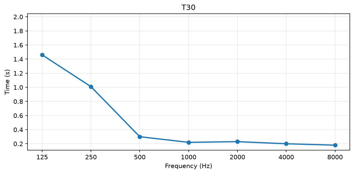
analyser.plot('T30')
Output
                   125     250     500    1000    2000    4000    8000
----------------------------------------------------------------------
EDT               1.64    0.62    0.31    0.18    0.24    0.22    0.18
T20               1.26    0.78    0.25    0.22    0.22    0.20    0.18
T30               1.46    1.01    0.30    0.22    0.23    0.20    0.18
C50              -4.21    2.99    8.93   13.80   13.24   15.46   16.57
C80               2.20    6.93   20.99   22.78   20.47   23.87   27.63
D50              27.49   66.54   88.66   96.00   95.48   97.23   97.84
DRR             -23.11   -7.71   -4.79   -5.89   -4.71   -5.75   -4.10
Ts                0.11    0.05    0.02    0.01    0.02    0.01    0.01
STI               0.54    0.67    0.84    0.89    0.87    0.88    0.90
G                30.04   23.35   21.51   20.08   19.86   20.84   18.87
SPL             130.04  123.35  121.51  120.08  119.86  120.84  118.87
LF                 nan     nan     nan     nan     nan     nan     nan
LFC                nan     nan     nan     nan     nan     nan     nan