Introduction to the Reachability Map
For workspace planning or robot path planning, it is useful to calculate and visualize the space of the robot’s reachability, depending on its attached tool, obstacles in the environment and its own kinematic and geometric constraints.
The ReachabilityMap is a collection of all valid IK solutions, i.e. poses that the end-effector can reach, at specified locations. The map is built by discretizing the robot’s environment, defining frames to be checked, and calculating the IK solutions for each frame.
The creation of this map depends on the availability of an analytical inverse kinematic solver for the used robot. Please checkout the kinematic backend for available robots.
Links
Example 01: reachability map 1D
Let’s consider the following (abstract) example:
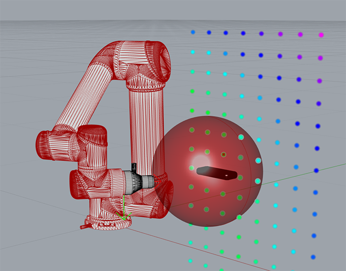
We have a UR5 and want the TCP of the robot to always orient itself towards a
defined position in front of the robot. Therefore, we define a (half-)sphere
with a certain radius and we evaluate points on this sphere. At each point, we then
create a plane whose normal vector points towards the center of this sphere. From these planes
we create frames for the robot’s TCP. The function is written as a generator
because the ReachabilityMap takes a Frame generator as input.
import math

from compas.geometry import Frame
from compas.geometry import Plane
from compas.geometry import Point
from compas.geometry import Sphere

# 1. Define frames on a sphere
sphere = Sphere((0.4, 0, 0), 0.15)

def points_on_sphere_generator(sphere):
    for theta_deg in range(0, 360, 20):
        for phi_deg in range(0, 90, 10):  # only half-sphere
            theta = math.radians(theta_deg)
            phi = math.radians(phi_deg)
            x = sphere.point.x + sphere.radius * math.cos(theta) * math.sin(phi)
            y = sphere.point.y + sphere.radius * math.sin(theta) * math.sin(phi)
            z = sphere.point.z + sphere.radius * math.cos(phi)
            point = Point(x, y, z)
            axis = sphere.point - point
            plane = Plane((x, y, z), axis)
            f = Frame.from_plane(plane)
            # for the old UR5 model from ROS Kinetic is zaxis the xaxis
            yield [Frame(f.point, f.zaxis, f.yaxis)]
Then we create a PyBulletClient (for collision checking), load the UR5 robot,
set the analytical IK solver and define options for the IK solver.
For simplicity, we do not add any tool or obstacles in the environment here, but in a
real robot cell, this will usually be the case.
# 2. Set up robot cell
from compas_fab.backends import AnalyticalInverseKinematics
from compas_fab.backends import PyBulletClient

with PyBulletClient(connection_type='direct') as client:
    # load robot and define settings
    robot = client.load_ur5(load_geometry=True)
    ik = AnalyticalInverseKinematics(client)
    client.inverse_kinematics = ik.inverse_kinematics
    options = {"solver": "ur5", "check_collision": True, "keep_order": True}
Now we create a ReachabilityMap. We calculate it passing the Frame
generator, the robot and the IK options. After calculation, we save the map as
json for later visualization in Rhino/GH.
>>> # 3. Create reachability map 1D
>>> map = ReachabilityMap()
>>> map.calculate(points_on_sphere_generator(sphere), robot, options)
>>> map.to_json(os.path.join(DATA, "reachability", "map1D.json"))
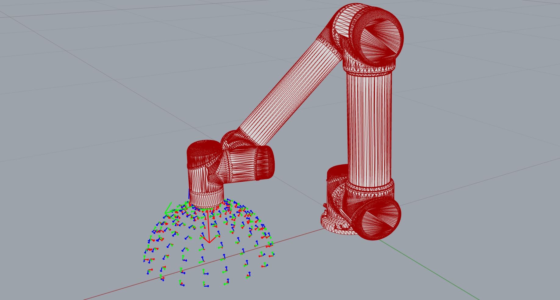
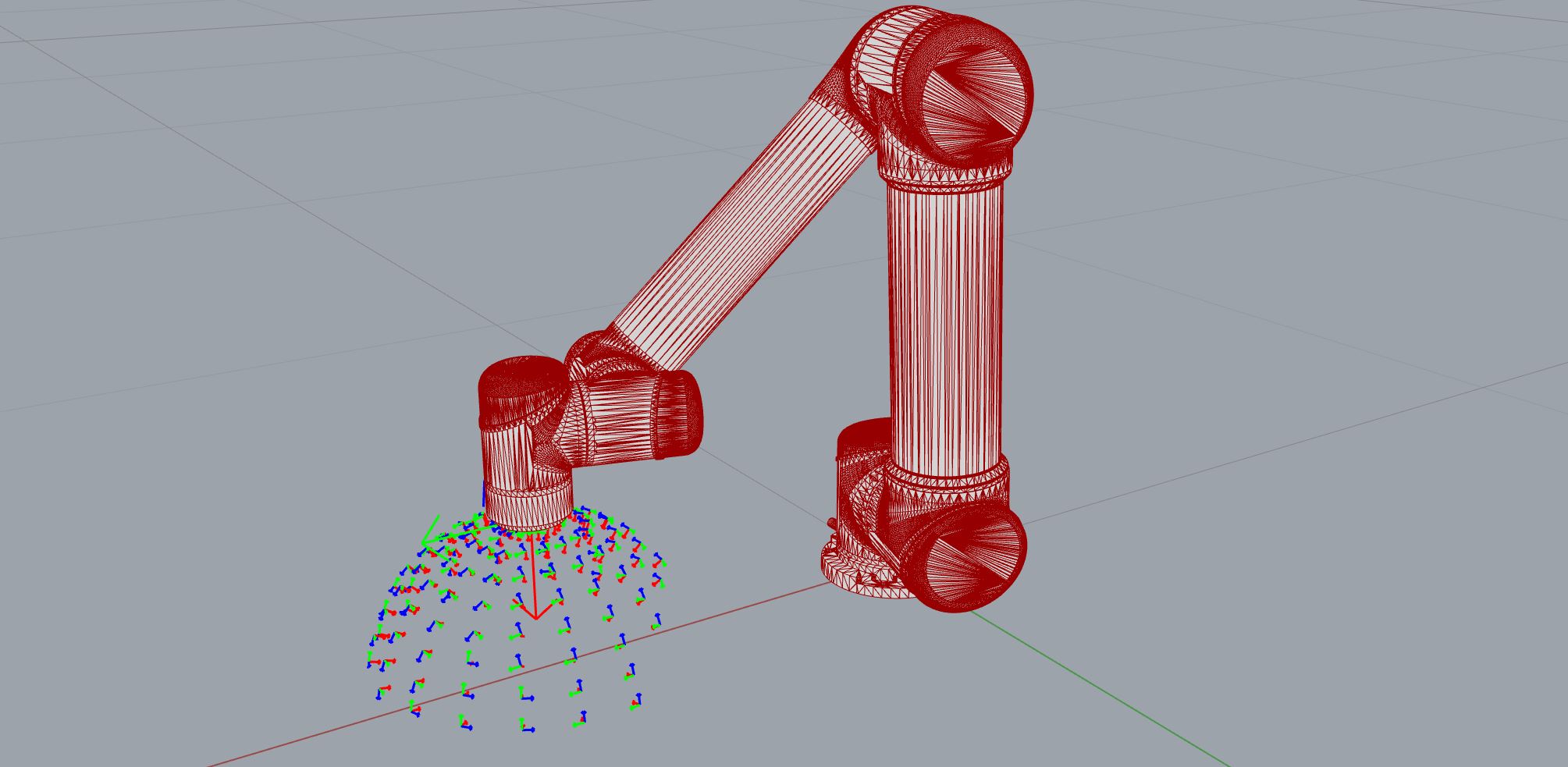
Visualization
We can source the reachability map from the json file and use the Artist to
visualize the saved frames by using the artist’s function draw_frames.
>>> map = ReachabilityMap.from_json(filepath)
>>> artist = Artist(map)
>>> frames = artist.draw_frames()
By default, the artist.draw() method returns points and colors for a point cloud,
where the points are the positions of the frames and the colors are calculated
from the score at the respective frame. The ReachabilityMap.score is
the number of valid IK solutions for a frame. The default colormap is ‘viridis’.
In the example below, the highest score is 4 (yellow) and the lowest score is 2 (violet).
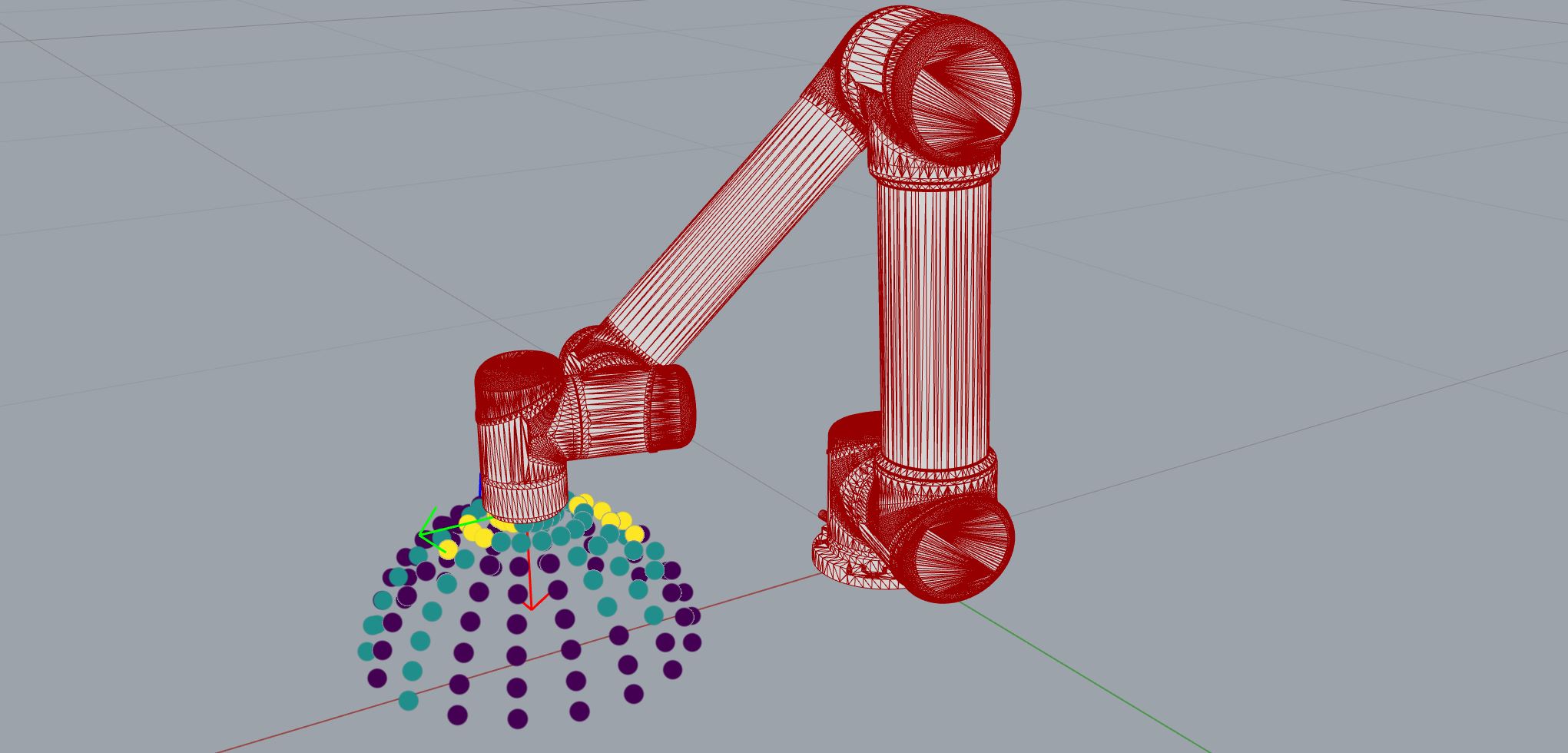
If you want to visualize the frames at a specific IK index (= number between 0-7), use the method
artist.draw_frames(ik_index=ik_index). If you compare the figure below
with the figure of draw_frames, you will see that a certain portion is not
reachable at the selected IK index.
Projects where the reachability map was applied
Adaptive Detailing
In this project, connections between structural elements are 3D printed in place,
directly on top of parts, i.e. collision objects. A ReachabilityMap was created
to capture the space where connections can be placed and ultimately find connecting
geometries that the robot can print in between these objects. Printing process
constraints can be included in the reachability map by choosing a meaningful
max_alpha in the DeviationVectorsGenerator.
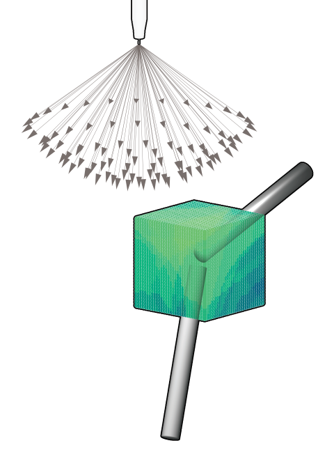
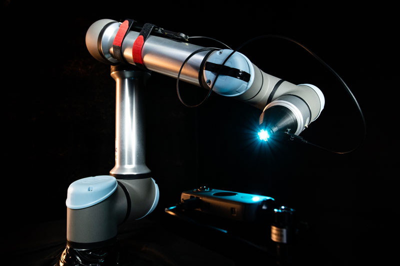
Robotic 360° Light Painting Workshop
This project served as inspiration for the presented examples 01-03. The robot TCP had to be oriented towards the 360° camera. The light paths were mapped on a hemisphere to maintain equal distance to the camera and little distortion of the designed paths. The reachability map was used to determine the best position and radius for the sphere with the UR5e robot model, the light tool, and the camera and tripods as collision objects.
|
|